Most people deeply interested in the topic of machine learning think it is synonymous with neural networks. In their current incarnation, neural networks seem to be versatile tools. By selecting the right type of neural network, the same tool, with small variations, might be able to solve most problems. This does not mean, though, that neural networks are the best (or even the right) tool to use for a given problem.
In this article, we'll look at a type of problem, exemplified by a little game, that can be solved easily with another technique called reinforcerment learning. We will look at the requirements, the implementation, and the model's advantages.
The game
This game can be played with pencil and paper, and it is good to gain first-hand experience before solving the problem with a program. This is a race game in which a track is traversed as quickly as possible while keeping the "car" on the track. The track and the position of the car are specified on a square grid. At any point in the game, the car has a location and speed. Speed includes (consistent with the definition of speed in physics) the direction. The movement rules are most easily explained graphically.

opensource.com
In these two different situations, the car's current position is represented by the red square and its previous position by the orange square. The distance between these two squares defines the speed of the car—(4,-1) in one case and (4,0) in the other—given a coordinate system with the first dimension going left to right and the second bottom to top.
The speed is measured in Manhattan distance by adding the absolute values of the two values: |4|+|-1|=5 and |4|+|0|=4.
The rules for the next move are: The length of the speed vector must change by at most one, up or down, and the values of the components of the speed vector must change by at most one each. As a result, there are up to seven possible locations the car can move to in the next step, represented in the diagrams by the green squares. If the current speed is one, the car could come to a standstill, but this is not useful since the goal is to complete the course as quickly as possible. This could be avoided by disallowing speed zero, which reduces the number of possible new locations in this case.
The track is the other limit. The car must not leave the track, and some (or all) of the possible new locations might be invalid given the speed of the car. The track does not have to be defined by straight lines and regular curves, and it can look like the following picture (or be even more complicated).
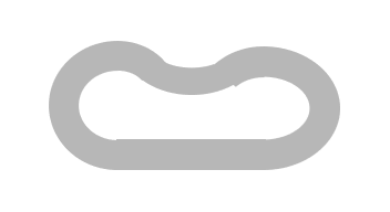
opensource.com
For this exercise, we must define a start/finish line on the track. The car starts on a location on this line, the initial speed is one (i.e., one step horizontally or vertically), and it must cross the line from the other side. In the example code, the track and the start line location are encoded in a lossless image file. The start position is given separately as a line on the start line.
Any successful race will cross the start/finish line without leaving the track. The best solution is the one that requires the fewest number of steps. There can, in most cases, be more than one possible solution, but this depends on the track and the starting condition.
Finding the solution
If we consider a traditional approach, where we determine a solution from the given state at the beginning, we quickly run into problems. There are simply too many possibilities.
The problem is that, to calculate the next step, all possible future steps must be taken into account. A closed formula of some sort probably cannot be formulated. This leaves recursive searching, which is very quickly non-practical, unless the track is very short. The combinatorial effort will be prohibitive.
For a non-trivial track, it is therefore probably necessary to settle for a probabilistic result.
Available information
In theory, it is possible to provide, at all steps on the way, information about all the future steps. As explained in the previous section, this is prohibitively expensive to do. To make the decision for the next step, we should restrict ourselves to a subset of that information—ideally, a very small subset. This will obviously not guarantee that we can find the best possible solution right away, but this is where machine learning techniques come in.
Q-learning
Here, we are looking at a machine learning technique called Q-learning, which is a specific reinforcement learning technique. It allows learning an action-value function, which is exactly what we want here: We want to know, in any situation, how to change the speed, and the quality of that move is the value. Deciding to use Q-learning does not, in itself, determine how the value is computed; that remains for the data scientist to decide.
We are not going into the details of the theory behind Q-learning here. Suffice it to say that it can find an optimal function for a large set of problems (for those interested, all Markov decision processes can be modeled). It is not necessary to have a model of the environment (i.e., in this case it is not necessary to model the entire track). We can just look at the immediate neighborhood of the car before and after the step, and determine a representation value or reward for each step.
The algorithm requires a representation of the current state: the position and the speed of the car. We want to determine the action in each state, i.e., the new speed and result from the new position. As written above, we need to assign a value to this, represented by a single number. What we get is the so-called Q-function:

opensource.com
We do not know anything about that function at the beginning, and we can initially return for all inputs a fixed, arbitrarily chosen value. Depending on the values that are later used in the learning phase, the initial value might have an influence on the learning speed.
Better values for Q are determined iteratively. This iteration step starts from a given state, determines an action (how this is done will be discussed below), and determines the reward. This information is then used to update the Q function:

opensource.com
Translated into words, this means that Q is updated for state st and action at by multiplying the old value with 1-α, and adding to it α times the sum of the reward for the step rt and γ times the maximum future value of Q (or an estimate of it). For the final states, we do not have to (and must not) update Q; we just set the reward appropriately. The multiplication with 1-α and α (respectively) guarantees that the value of Q is limited by the choice of the initial value and the reward for the final states.
The value γ is a so-called hyperparameter of the learning algorithm. In this case, it is the discount factor, a term used in similar situations (e.g., financial math). It means that if the reward at a future state is r, its value in the current state has to be discounted, since the reward can only be collected after one or more additional steps. Each step discounts by the factor 0<γ<1. Finding the right value for γ is part of developing the model.
With this description, it should already be possible to see how the model learning can happen. We start in a given state, pick an action, compute the reward, and determine the optimum reward for actions starting in the new state. Using all this information, we update the Q function for the current state and proceed from there. There are a few things to note:
- In our example, there are at most seven possible actions in each state; less if the track is limiting the movement. The representation of Q is therefore not particularly problematic.
- Initially, all values of Q—except for the final states—are arbitrarily initialized. Therefore, the maximum values of the future steps do not differ much at the outset. Only states where the next step leads to a final state will initially find a big future reward. Repeating the iteration, over and over from the beginning, will propagate the high reward values to the earlier states on the path that lead to the goal. The paths/states that do not lead to the goal will never have a high future reward.
There is one remaining detail to consider: how to choose the next step during the learning phase. Since many steps might be needed to reach the goal, it is undesirable to choose the next step randomly, which offers a low probability that the goal will be reached.
High values of Q can be used to guide the selection. But always choosing the action with the highest reward might mean better alternatives are never explored. Therefore, we need a mix: with a given probability ε, we choose a random (valid) next state. Otherwise we pick one among the possible states with the highest Q value. ε becomes another hyperparameter of the algorithm, which selects how much exploration happens versus how far a known good path is followed.
Alternatively, it is possible to use the initial value for Q to encourage exploration. Using a high value will ensure that the states are eventually explored, and those that do not lead to the goal will over time see their Q value lowered. The choice for the initial value is crucial here, since it must not be dwarfed by the reward values.
Once the model is sufficiently trained, we can determine the optimal step in any state by looking for the action with the highest reward, then continue to do the same until the goal is reached. The algorithm is guaranteed to find an optimal solution eventually, but this might take time, and prematurely testing for a solution might not lead to a correct result: i.e., the chain s1→s2→…→sn might not lead to a final state when the action at with the best Q value is chosen each time. This is something to keep in mind when using the model.
Applying Q-learning
Now we are ready to apply Q-learning to the problem of racing the car around the track. To apply the algorithm, we need a way to compute the reward.
- If the next step would leave the track, the reward is minimal.
- A new state that is closer to the goal has a higher reward.
- A new state with a higher speed has a higher reward.
The last two aspects of the of the reward are designed to give a higher value in case the goal can be reached quicker because the goal is closer, the speed is higher, or both. The benefits for distance to the goal and for speed should be additive.
There is still a lot of flexibility in defining the function. The following is one possible way.
def getr(d1, d2, va, Qgoal):
    if d1 < 0 or d2 < 0 or d1 - d2 > va:
        return None

    if d1 < d2:
        if d1 <= va and d2 > 5 * va:
            return Qgoal
        return (d1 - d2) - (va >> 1) / (d1 - d2)
    else:
        return (1 + d1 - d2) * va
Even those not familiar with Python should be able to understand the code. The parameters d1 and d2 are the distances to the goal for the current and next position, and va is the current speed. The absolute values is not used except to check for invalid positions. Only the difference is used to compute the value of the reward and therefore it does not matter how these values are defined. They can use only local information. The direction to the goal line is known because you know the last position, and you can count how many steps are taken in the right direction.
The values of d1 and d2 are negative for all locations outside the track. If this is detected (or in other invalid situations), the value None is returned, indicating that this move is not possible and does not have to investigated further. The formula accounts for the case that the new position is further away from the goal, but if the speed is high enough, it is still worth something. The main rule is the last one, which scales the reward with both the reduced distance to the goal line and the speed. This version of the scoring is by no means ideal or the only one. It is just one example. Part of the development process of the model is it to try more and different versions of this function.
This function is called for the different states the car is in. Now we have to discuss how these different states are determined.
Inner learning loop
In the inner loop, we have to determine the next state by determining which of the seven possible speeds the car can have in the next step and, based on this and the current position, which are the acceptable locations on the track. Then we use the algorithm discussed above to select one of the possible next steps. The resulting code can look like this:
  co = (start[0] + startspeed[0], start[1] + startspeed[1])
  speed = startspeed
  aspeed = absspeed(speed)
  nextspeeds = possible_speeds(speed)
  curdist = dist[co[0]][co[1]]
  scores = score[co[0]][co[1]]
  known = known_speeds(scores, nextspeeds)
  bestscore = Qfail
  bestspeeds = []
  for s in known:
    thisscore = scores[s]
    if thisscore == bestscore:
      bestspeeds.append(s)
    elif thisscore > bestscore:
      bestscore = thisscore
      bestspeeds = [ s ]
  if bestscore < Q0 and len(known) != len(nextspeeds):
    bestscore = Q0
    bestspeeds = set(nextspeeds) - set(known)
  path = [ ]
  reached_goal = False

  while True:
    path.append((speed, co))

    if random.random() < epsilon:
      nextspeed = random.sample(nextspeeds, 1)[0]
    else:
      # Pick according to current score
      nextspeed = random.sample(bestspeeds, 1)[0]

    nextco = (co[0] + nextspeed[0], co[1] + nextspeed[1])
    nextdist = dist[nextco[0]][nextco[1]]
    nextaspeed = absspeed(nextspeed)

    r = getr(curdist, nextdist, nextaspeed, Qgoal)
    if not r:
      # crash
      score[co[0]][co[1]][nextspeed] = Qfail
      break

    if curdist <= aspeed and nextdist > 10 * aspeed:
      nextbestscore = Qgoal
      reached_goal = True
    else:
      scores = score[nextco[0]][nextco[1]]
      speedspp = possible_speeds(nextspeed)
      known = known_speeds(scores, speedspp)
      bestscore = Qfail
      bestspeeds = []
      for s in known:
        thisscore = scores[s]
        if thisscore == bestscore:
          bestspeeds.append(s)
        elif thisscore > bestscore:
          bestscore = thisscore
          bestspeeds = [ s ]
        if bestscore < Q0 and len(known) != len(speedspp):
            bestscore = Q0
            bestspeeds = set(speedspp) - set(known)

    oldval = score[co[0]][co[1]][nextspeed] if nextspeed in
                score[co[0]][co[1]] else Q0
    score[co[0]][co[1]][nextspeed] = (1 - alpha) * oldval +
                                     alpha * (r + gamma * bestscore)

    if reached_goal or len(path) > 5 * tracklen:
      break

    co = nextco
    speed = nextspeed
    aspeed = nextaspeed
    nextspeeds = speedspp
    curdist = nextdist
This is all of the code that creates a path from the fixed starting point (start) and starting speed (startspeed) until the point the goal line is crossed or the car leaves the track. In preparation for the loop, a whole set of variables is computed. This happens because, in the second part of the loop, these variables are computed for the next step. We can reuse the work.
The variables nextspeeds, which is a list of the possible speeds for the next step, and bestspeeds, which is a list of the speeds that lead to states with the highest scores, are the main initialization needed.
In the loop, first the new position is recorded in path. It follows the determination of the possible speeds along the rules of the game, making sure the speed does not drop to zero. All possible new speeds are stored in the list nextspeeds.
From this list, one speed is selected. With a probability represented by epsilon, a random value is selected. Otherwise one of the next states with the best score is chosen. This is also a choice between multiple possibilities, in case there are multiple states with the same score.
The value for epsilon must be sufficiently small to allow trying to improve previously found good sequences. Following along, the first n best scores (because no random choice is made) have the probability of (1 - ε)n, which for ε=5% means 6 in 1,000 attempts make it all the way through. That might not be sufficient in case long paths have to be discovered. ε is an important hyperparameter.
Once the new speed is selected, the next coordinate of the car is computed in newco.
After that, the score for the current position is updated. The score variable is indexed by the coordinate and the selected speed. The reward is computed by calling getr, which we saw in the previous section. If the coordinates fall outside the track, we assign a negative score and terminate the loop. The value used for the negative reward is also a hyperparameter.
What follows is an implementation of the Q-function update we saw above. We determine from all the possible next states the one with the best score, and then use the hyperparameters α and γ to update the score. The only complication is that speed values are not yet known in the score array, and then we have to use the value Q0.
Discussion
That is all. No knowledge of the problem had to be encoded to solve it. The only detail that ties the implementation to the problem is the implementation of the getr function, which provides environmental information. As we have seen, the information used is local; no global information about the problem is used. The implementation uses the fact that only a small number of actions are possible in each state, and the implementation therefore can rely on a dictionary implementation. This might not be the case for all possible problems you may want to use this machine learning algorithm for. Aside from that, the implementation can be reused.
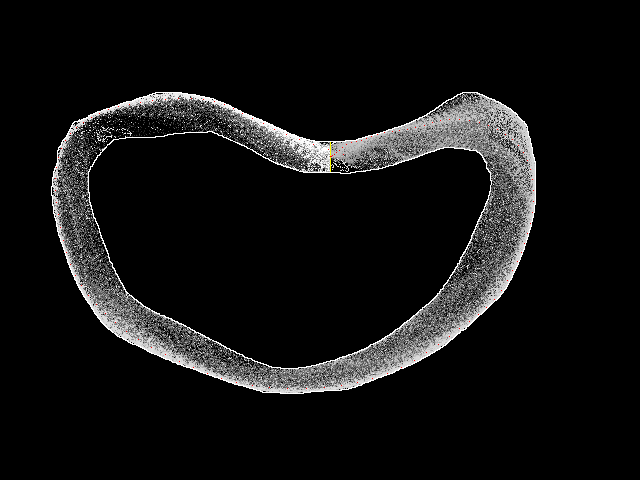
The following is the output of the implementation after 4-million runs.
opensource.com
The track's outline is clearly visible. Inside, using different levels of gray, the best score among the individual positions on the track is shown. This representation omits a lot of information, since the actions at each position of the track encompass possibly many different speeds, and only one value is displayed. The graphic is still useful.
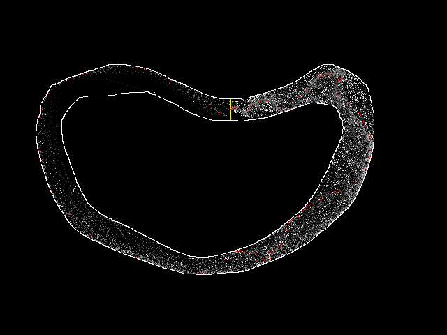
The red points (barely visible here, but you can zoom in on the image in this project's GitHub) make up the best path that comprises the "solution" we are looking for. It is not guaranteed to be the best solution unless the algorithm runs for an infinite amount of time. The solution is guaranteed to get better over time—and the one in the example does not look so bad. It would not be easy to write a specific algorithm to better solve the problem. To see the progress the algorithm made, we can look at the state of the program after fewer runs, such as in the case below after just 20,000 runs.
opensource.com
We can see that a solution has been found, but it is not really good. The steps taken do not come in straight lines or regular curves. Instead, the red line makes all kinds of curves. This is understandable, since at the beginning the algorithm basically performs a random walk, and if some steps do not immediately result in a crash, they will receive a positive score. Once this is done, the algorithm mostly (determined by ε) follows known-good paths. Only once in a while will the algorithm step off these "good" paths and try something else. If those steps happen to be in the right direction, they will easily overpower the previous good paths, and the entire path taken by the car will become more and more straight.
Try it yourself
There are a lot of ways to influence the learning algorithm, from hyperparameters like ε, α, γ, and so forth, to a different implementation of the getr function. You can try it yourself by starting from the code shown in this article, which can be downloaded from track-rl on GitHub





Comments are closed.