If you made through part 1, congrats! You have the patience it takes to format data. In that article, I cleaned up my National Football League data set using a few Python libraries and some basic football knowledge. Picking up where I left off, it's time to take a closer look at my data set.
Data analysis
I'm going to create a final dataframe that contains only the data fields I want to use. These mostly will be the data fields I created when transforming columns in addition to down and distance (aka yardsToGo).
df_final = df[['down','yardsToGo', 'yardsToEndzone', 'rb_count', 'te_count', 'wr_count', 'ol_count',
               'db_count', 'secondsLeftInHalf', 'half', 'numericPlayType', 'numericFormation', 'play_type']]
Now I want to spot check my data using dataframe.describe(). It sort of summarizes the data in the dataframe and makes it easier to spot any unusual values.
print(df_final.describe(include='all'))

Most everything looks good, except yardsToEndzone has a lower count than the rest of the columns. The dataframe.describe() documentation defines the count return value as the "number of non-NA/null observations." I need to check whether I have null yard-line values.
print(df.yardlineNumber.unique())

Why is there a nan value? Why do I seem to be missing a 50-yard line? If I didn't know any better, I'd say my undiluted data from the NFL dump doesn't actually use the 50-yard line as a value and instead marks it as nan.
Here are some play descriptions for a few of the plays where the yard-line value is NA:

It seems my hypothesis is correct. Each play description's ending yard line and yards gained come out to 50. Perfect (why?!). I'll map these nan values to 50 by adding a single line before the yards_to_endzone function from last time.
df['yardlineNumber'] = df['yardlineNumber'].fillna(50)
Running df_final.describe() again, I now have uniform counts across the board. Who knew so much of this practice was just grinding through data? I liked it better when it had an air of mysticism about it.
It's time to start my visualization. Seaborn is a helpful library for plotting data, and I already imported it in part 1.
Play type
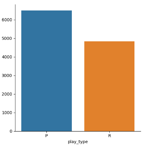
How many plays are passing plays vs. running plays in the full data set?
sns.catplot(x='play_type', kind='count', data=df_final, orient='h')
plt.show()

It looks like there are about 1,000 more passing plays than running plays. This is important because it means the distribution between both play types is not a 50/50 split. By default, there should be slightly more passing plays than running plays for every split.
Downs
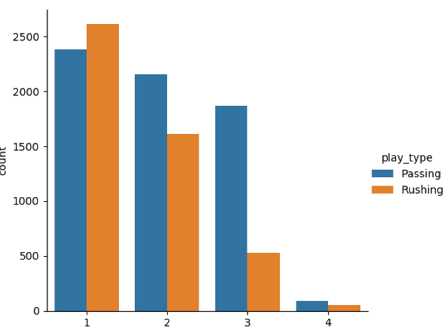
A down is a period where a team can attempt a play. In the NFL, an offense gets four play attempts (called "downs") to gain a specified number of yards (usually starting with 10 yards); if it doesn't, it has to give the ball to the opponent. Is there a specific down that tends to have more passes or runs (also called rushes)?
sns.catplot(x="down", kind="count", hue='play_type', data=df_final);
plt.show()

Third downs have significantly more passing plays than running plays but, given the initial data distribution, this is probably meaningless.
Regression
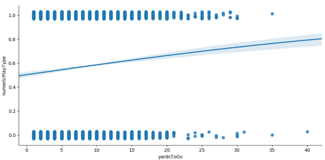
I can use the numericPlayType column to my advantage and create a regression plot to see if there are any trends.
sns.lmplot(x="yardsToGo", y="numericPlayType", data=df_final, y_jitter=.03, logistic=True, aspect=2);
plt.show()

This is a basic regression chart that says the larger the value of yards to go, the larger the numeric play type will be. With a play type of 0 for running and 1 for passing, this means that the more distance there is to cover, the more likely the play will be a passing type.
Model training
I'm going to use XGBoost for training; it requires input data to be all numeric (so I have to drop the play_type column I used in my visualizations). I also need to split my data into training, validation, and testing subsets.
train_df, validation_df, test_df = np.split(df_final.sample(frac=1), [int(0.7 * len(df)), int(0.9 * len(df))])


print("Training size is %d, validation size is %d, test size is %d" % (len(train_df),
                                                                           len(validation_df),
                                                                           len(test_df)))
XGBoost takes data in a particular data structure format, which I can create using the DMatrix function. Basically, I'll declare numericPlayType as the label I want to predict, so I'll feed it a clean set of data without that column.
train_clean_df = train_df.drop(columns=['numericPlayType'])
d_train = xgb.DMatrix(train_clean_df, label=train_df['numericPlayType'],
                      feature_names=list(train_clean_df))


val_clean_df = validation_df.drop(columns =['numericPlayType'])
d_val = xgb.DMatrix(val_clean_df, label=validation_df['numericPlayType'],
                    feature_names=list(val_clean_df))


eval_list = [(d_train, 'train'), (d_val, 'eval')]
results = {}
The remaining setup requires some parameter adjustments. Without getting too into the weeds, predicting run/pass is a binary problem, and I should set the objective to binary.logistic. For more information about all of XGBoost's parameters, consult its documentation.
param = {
    'objective': 'binary:logistic',
    'eval_metric': 'auc',
    'max_depth': 5,
    'eta': 0.2,
    'rate_drop': 0.2,
    'min_child_weight': 6,
    'gamma': 4,
    'subsample': 0.8,
    'alpha': 0.1
}
Several unsavory insults directed at my PC and a two-part series later, (sobs in Python), I am officially ready to train my model! I'm going to set an early stopping round, meaning that if the evaluation metric for model training declines after eight rounds, I will end the training. This helps prevent overfitting. The prediction results are represented as a probability that the result will be a 1 (passing play).
num_round = 250
xgb_model = xgb.train(param, d_train, num_round, eval_list, early_stopping_rounds=8, evals_result=results)


test_clean_df = test_df.drop(columns=['numericPlayType'])
d_test = xgb.DMatrix(test_clean_df, label=test_df['numericPlayType'],
                     feature_names=list(test_clean_df))


actual = test_df['numericPlayType']
predictions = xgb_model.predict(d_test)
print(predictions[:5])
opensource.com
I want to see how accurate my model is using my rounded predictions (to 0 or 1) and scikit-learn's metrics package.
rounded_predictions = np.round(predictions)

accuracy = metrics.accuracy_score(actual, rounded_predictions)

print("Metrics:\nAccuracy: %.4f" % (accuracy))
Well, 75% accuracy is not bad for a first try at training. For those familiar with the NFL, you can call me the next Sean McVay. (This is funny, trust me.)
Using Python and its vast repertoire of libraries and models, I could reasonably predict the play type outcome. However, there are still some factors I did not consider. What effect does defense personnel have on play type? What about score differential at the time of the play? I suppose there is always room to go over your data and improve. Alas, this is the life of a programmer turned data scientist. Time to consider early retirement.


1 Comment