Data science is a domain of knowledge that spans programming languages. Some are well-known for solving problems in this space, while others are lesser-known. This article will help you become familiar with doing data science with some popular languages.
Choosing Python and GNU Octave for data science
Every so often, I try to learn a new programming language. Why? It is mostly a combination of boredom with the old ways and curiosity about the new ways. When I started programming, the only language I knew was C. Life was hard and dangerous in those years, as I had to manually allocate memory, manage pointers, and remember to free memory.
Then a friend suggested I try Python, and life became much easier. Programs became much slower, but I did not have to suffer through writing analysis software. However, I soon realized that each language was more suitable than others for some applications. I later studied some other languages, and each one brought some new bit of enlightenment. Discovering new programming styles let me backport some solutions to other languages, and everything became much more interesting.
To get a feeling for a new programming language (and its documentation), I always start by writing some example programs that perform a task I know well. To that ends, I will explain how to write a program in Python and GNU Octave for a particular task you could classify as data science. If you are already familiar with one of the languages, start with that one and go through the others to look for similarities and differences. It is not intended to be an exhaustive comparison of the languages, just a little showcase.
All of the programs are meant to be run on the command line, not with a graphical user interface (GUI). The full examples are available in the polyglot_fit repository.
The programming task
The program you will write in this series:
- Reads data from a CSV file
- Interpolates the data with a straight line (i.e., f(x)=m ⋅ x + q)
- Plots the result to an image file
This is a common situation that many data scientists have encountered. The example data is the first set of Anscombe's quartet, shown in the table below. This is a set of artificially constructed data that gives the same results when fitted with a straight line, but their plots are very different. The data file is a text file with tabs as column separators and a few lines as a header. This task will use only the first set (i.e., the first two columns).
| I | II | III | IV | ||||
|---|---|---|---|---|---|---|---|
| x | y | x | y | x | y | x | y |
| 10.0 | 8.04 | 10.0 | 9.14 | 10.0 | 7.46 | 8.0 | 6.58 |
| 8.0 | 6.95 | 8.0 | 8.14 | 8.0 | 6.77 | 8.0 | 5.76 |
| 13.0 | 7.58 | 13.0 | 8.74 | 13.0 | 12.74 | 8.0 | 7.71 |
| 9.0 | 8.81 | 9.0 | 8.77 | 9.0 | 7.11 | 8.0 | 8.84 |
| 11.0 | 8.33 | 11.0 | 9.26 | 11.0 | 7.81 | 8.0 | 8.47 |
| 14.0 | 9.96 | 14.0 | 8.10 | 14.0 | 8.84 | 8.0 | 7.04 |
| 6.0 | 7.24 | 6.0 | 6.13 | 6.0 | 6.08 | 8.0 | 5.25 |
| 4.0 | 4.26 | 4.0 | 3.10 | 4.0 | 5.39 | 19.0 | 12.50 |
| 12.0 | 10.84 | 12.0 | 9.13 | 12.0 | 8.15 | 8.0 | 5.56 |
| 7.0 | 4.82 | 7.0 | 7.26 | 7.0 | 6.42 | 8.0 | 7.91 |
| 5.0 | 5.68 | 5.0 | 4.74 | 5.0 | 5.73 | 8.0 | 6.89 |
The Python way
Python is a general-purpose programming language that is among the most popular languages in use today (as evidenced by findings from the TIOBE index, RedMonk Programming Language Rankings, Popularity of Programming Language Index, State of the Octoverse of GitHub, and other sources). It is an interpreted language; therefore, the source code is read and evaluated by a program that executes the instructions. It has a comprehensive standard library and is generally very pleasant to use (I have no reference for this last statement; it is just my humble opinion).
Installation
To develop with Python, you need the interpreter and a few libraries. The minimum requirements are:
- NumPy for convenient array and matrices manipulation
- SciPy for scientific calculations
- Matplotlib for plotting
Installing them in Fedora is easy:
sudo dnf install python3 python3-numpy python3-scipy python3-matplotlibCommenting code
In Python, comments are achieved by putting a # at the beginning of the line, and the rest of the line will be discarded by the interpreter:
# This is a comment ignored by the interpreter.The fitting_python.py example uses comments to insert licensing information in the source code, and the first line is a special comment that enables the script to be executed on the command line:
#! /usr/bin/env python3This line informs the command-line interpreter that the script needs to be executed by the program python3.
Required libraries
Libraries and modules can be imported in Python as an object (as in the first line in the example) with all the functions and members of the library. There is a convenient option to rename them with a custom label by using the as specification:
import numpy as np
from scipy import stats
import matplotlib.pyplot as plt
You may also decide to import only a submodule (as in the second and third lines). The syntax has two (more or less) equivalent options: import module.submodule and from module import submodule.
Defining variables
Python's variables are declared the first time a value is assigned to them:
input_file_name = "anscombe.csv"
delimiter = "\t"
skip_header = 3
column_x = 0
column_y = 1
The variable types are inferred by the value that is assigned to the variable. There are no variables with constant values unless they are declared in a module and can only be read. Idiomatically, variables that should not be modified should be named in uppercase.
Printing output
Running the programs through the command line means that the output is just printed on the terminal. Python has the print() function that, by default, prints its argument and adds a newline at the end of the output:
print("#### Anscombe's first set with Python ####")It is possible to combine the print() function with the formatting power of the string class in Python. Strings have the format method that can be used to add some formatted text to the string itself. For instance, it is possible to add a formatted float number, e.g.:
print("Slope: {:f}".format(slope))Reading data
Reading CSV files is very easy with NumPy and the function genfromtxt(), which generates a NumPy array:
data = np.genfromtxt(input_file_name, delimiter = delimiter, skip_header = skip_header)In Python, a function can have a variable number of arguments, and you can have it pass a subset by specifying the desired ones. Arrays are very powerful matrix-like objects that can be easily sliced into smaller arrays:
x = data[:, column_x]
y = data[:, column_y]
The colons select the whole range, and they can also be used to select a subrange. For instance, to select the first two rows of the array, you would use:
first_two_rows = data[0:1, :]Fitting data
SciPy provides convenient functions for data fitting, such as the linregress() function. This function provides some significant values related to the fit, such as the slope, intercept, and the correlation coefficient of the two datasets:
slope, intercept, r_value, p_value, std_err = stats.linregress(x, y)

print("Slope: {:f}".format(slope))
print("Intercept: {:f}".format(intercept))
print("Correlation coefficient: {:f}".format(r_value))
Since linregress() provides several pieces of information, the result can be saved to several variables at the same time.
Plotting
The Matplotlib library plots only data points; therefore, you should define the points you want to plot. The x and y arrays were already defined, so you can directly plot them, but you also need data points that will represent the straight line.
fit_x = np.linspace(x.min() - 1, x.max() + 1, 100)The linspace() function conveniently generates a set of equally spaced values between two values. The ordinates can be easily calculated by exploiting the powerful NumPy arrays, which can be used in a formula as if they were ordinary numeric variables:
fit_y = slope * fit_x + interceptThe formula is applied element-by-element on the array; therefore, the result has the same number of entries in the initial array.
To create the plot, first, define a figure object that will contain all the graphics:
fig_width = 7 #inch
fig_height = fig_width / 16 * 9 #inch
fig_dpi = 100

fig = plt.figure(figsize = (fig_width, fig_height), dpi = fig_dpi)
Several plots can be drawn on a figure; in Matplotlib, the plots are called axes. This example defines a single axis object to plot the data points:
ax = fig.add_subplot(111)

ax.plot(fit_x, fit_y, label = "Fit", linestyle = '-')
ax.plot(x, y, label = "Data", marker = '.', linestyle = '')

ax.legend()
ax.set_xlim(min(x) - 1, max(x) + 1)
ax.set_ylim(min(y) - 1, max(y) + 1)
ax.set_xlabel('x')
ax.set_ylabel('y')
Save the figure to a PNG image file with:
fig.savefig('fit_python.png')If you want to display (instead of saving) the plot, call:
plt.show()This example references all the objects used in the plotting section: it defines the object fig and the object ax. This technicality is not necessary, as the plt object can be used directly to plot the datasets. The Matplotlib tutorial shows an interface such as:
plt.plot(fit_x, fit_y)Frankly, I do not like this approach because it hides the non-trivial interactions that happen between the various objects. Unfortunately, sometimes the official examples are a bit confusing because they tend to use different approaches. Referencing graphical objects is not necessary in this simple example, but it becomes important in more complex ones (such as when embedding plots in GUIs).
Results
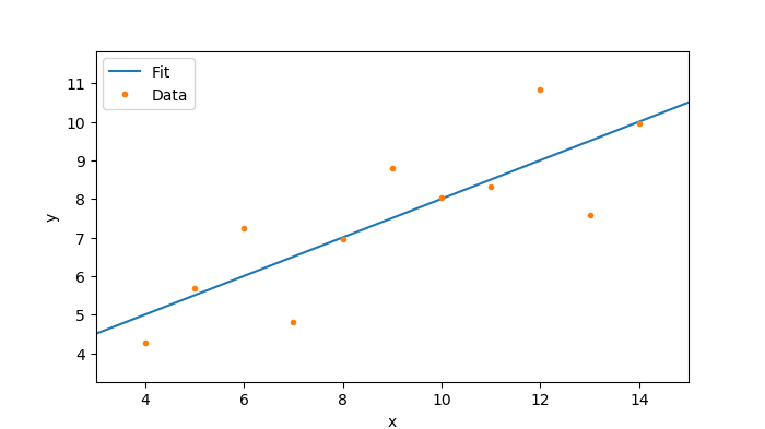
The output on the command line is:
#### Anscombe's first set with Python ####
Slope: 0.500091
Intercept: 3.000091
Correlation coefficient: 0.816421
Here is the image Matplotlib generates.

The GNU Octave way
The GNU Octave language is primarily intended for numerical computations. It offers a simple syntax for manipulating vectors and matrices and has some powerful plotting facilities. It is an interpreted language like Python. Since Octave's syntax is mostly compatible with MATLAB, it is often described as a free alternative to MATLAB. Octave is not listed among the most popular programming languages, but MATLAB is, so Octave is rather popular in a sense. MATLAB predates NumPy, and I have the feeling that it was inspired by the former. While you go through the example, you will see the analogies.
Installation
The fitting_octave.m example only needs the basic Octave package, making the installation in Fedora rather simple:
sudo dnf install octaveCommenting code
In Octave, you can add comments to code with the percent symbol (%), and you can also use # if MATLAB compatibility is not needed. The option to use # allows you to write the same special comment line from the Python example to execute the script directly on the command line.
Necessary libraries
Everything used in this example is contained in the basic package, so you do not need to load any new libraries. If you need a library, the syntax is pkg load module. This command adds the module's functions to the list of available functions. In this regard, Python has more flexibility.
Defining variables
Variables are defined with pretty much the same syntax as Python:
input_file_name = "anscombe.csv";
delimiter = "\t";
skip_header = 3;
column_x = 1;
column_y = 2;
Note that the end of the line has a semicolon; this is not necessary, but it suppresses the output of the results of the line. Without a semicolon, the interpreter would print the result of the expression:
octave:1> input_file_name = "anscombe.csv"
input_file_name = anscombe.csv
octave:2> sqrt(2)
ans =  1.4142
Printing output
The powerful function printf() is used to print on the terminal. Unlike in Python, the printf() function does not automatically add a newline at the end of the printed string, so you have to add it. The first argument is a string that can contain format information for the other arguments to be passed to the function, such as:
printf("Slope: %f\n", slope);In Python, the formatting is built into the string itself, but in Octave, it is specific to the printf() function.
Reading data
The dlmread() function can read text files structured like CSV files:
data = dlmread(input_file_name, delimiter, skip_header, 0);The result is a matrix object, which is one of the fundamental data types in Octave. Matrices may be sliced with a syntax similar to Python:
x = data(:, column_x);
y = data(:, column_y);
The fundamental difference is that the indexes start at one instead of zero. Therefore, in the example, the
x column is column number one.
Fitting data
To fit the data with a straight line, you can use the polyfit() function. It fits the input data with a polynomial, so you just need to use a polynomial of order one:
p = polyfit(x, y, 1);

slope = p(1);
intercept = p(2);
The result is a matrix with the polynomial coefficients; therefore, it selects the first two indexes. To determine the correlation coefficient, use the corr() function:
r_value = corr(x, y);Finally, print the results with the printf() function:
printf("Slope: %f\n", slope);
printf("Intercept: %f\n", intercept);
printf("Correlation coefficient: %f\n", r_value);
Plotting
As in the Matplotlib example, you first need to create a dataset that represents the fitted line:
fit_x = linspace(min(x) - 1, max(x) + 1, 100);
fit_y = slope * fit_x + intercept;
The analogy with NumPy is also evident here, as it uses the linspace() function that behaves just like the Python's equivalent version.
Again, as with Matplotlib, create a figure object first, then create an axes object to hold the plots:
fig_width = 7; %inch
fig_height = fig_width / 16 * 9; %inch
fig_dpi = 100;

fig = figure("units", "inches",
             "position", [1, 1, fig_width, fig_height]);

ax = axes("parent", fig);

set(ax, "fontsize", 14);
set(ax, "linewidth", 2);
To set properties of the axes object, use the set() function. The interface is rather confusing, though, as the function expects a comma-separated list of property and value pairs. These pairs are just a succession of a string representing the property name and a second object representing the value for that property. There are also other functions to set various properties:
xlim(ax, [min(x) - 1, max(x) + 1]);
ylim(ax, [min(y) - 1, max(y) + 1]);
xlabel(ax, 'x');
ylabel(ax, 'y');
Plotting is achieved with the plot() function. The default behavior is that each call resets the axes, so you need to use the function hold().
hold(ax, "on");

plot(ax, fit_x, fit_y,
     "marker", "none",
     "linestyle", "-",
     "linewidth", 2);
plot(ax, x, y,
     "marker", ".",
     "markersize", 20,
     "linestyle", "none");

hold(ax, "off");
Also, it is possible in the plot() function to add the property and value pairs. The legend must be created separately, and the labels should be stated manually:
lg = legend(ax, "Fit", "Data");
set(lg, "location", "northwest");
Finally, save the output to a PNG image:
image_size = sprintf("-S%f,%f", fig_width * fig_dpi, fig_height * fig_dpi);
image_resolution = sprintf("-r%f,%f", fig_dpi);

print(fig, 'fit_octave.png',
      '-dpng',
      image_size,
      image_resolution);
Confusingly, in this case, the options are passed as a single string with the property name and the value. Since in Octave strings do not have the formatting facilities of Python, you must use the sprintf() function. It behaves just like the printf() function, but its result is not printed, rather it is returned as a string.
In this example, as in the Python one, the graphical objects are referenced to keep their interactions evident. If Python's documentation in this regard is a little bit confusing, Octave's documentation is even worse. Most of the examples I found did not care about referencing the objects; instead, they rely on the fact that the plotting commands act on the currently active figure. A global root graphics object keeps track of the existing figures and axes.
Results
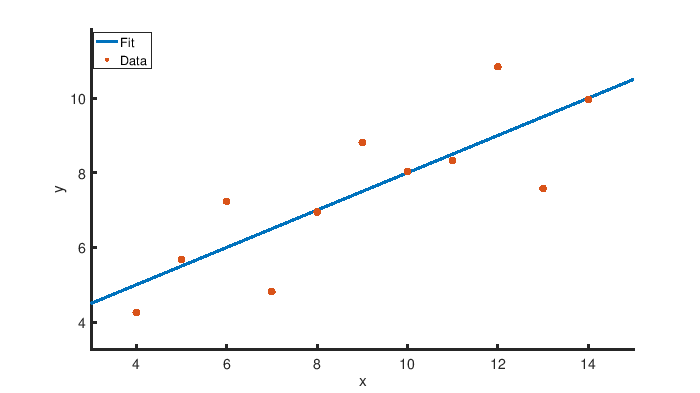
The resulting output on the command line is:
#### Anscombe's first set with Octave ####
Slope: 0.500091
Intercept: 3.000091
Correlation coefficient: 0.816421
And this shows the resulting image generated with Octave.

Next up
Both Python and GNU Octave can plot the same information, though they differ in how they get there. If you're looking to explore other languages to complete similar tasks, I highly recommend looking at Rosetta Code. It's a marvelous resource to see how to solve the same problems in many languages.
What language do you like to plot data in? Share your thoughts in the comments.


2 Comments